Correlation & Regression
Almost every interesting question in the world is a question about two things at once: does studying more raise a score, does a heavier dose lower a symptom, does price move with square footage. Correlation and regression are the two tools that answer those questions honestly. Correlation puts a single number on how tightly two quantitative variables track each other; regression draws the one straight line that fits the cloud of points better than any other line could, and lets you use it to predict. Neither tool requires you to be fast at arithmetic — every formula in this chapter is built from things you already know, means and standard deviations. What they do require is care in interpretation, because this is the corner of statistics where confident people say wrong things most often.
By the end of this chapter you can
- Build and read a scatterplot, and describe a relationship by its form, direction, and strength.
- Place the explanatory and response variables on the correct axes.
- Compute the correlation coefficient r by hand from deviations, and interpret its size and sign correctly.
- State the cautions on r — linearity only, outlier sensitivity, restricted range, and the fact that correlation is not causation.
- Find the least-squares regression line, and explain exactly what quantity "least squares" makes smallest.
- Interpret the slope and intercept in the units of the problem, without smuggling in a causal claim.
- Compute residuals and r2, and read a residual plot for curvature, spread, and outliers.
- Use the line to predict, and recognize when a prediction is illegitimate extrapolation.
- State the assumptions behind inference on the slope, and phrase a p-value and a confidence interval correctly.
Section 1Scatterplots
One dot, one individual, two measurements
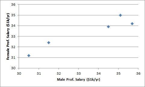
Everything up to this point in the book has described one variable at a time: the mean of a set of scores, the spread of a set of blood pressures. A scatterplot is the first graph that shows two quantitative variables measured on the same individuals. Each individual contributes a single dot, positioned by its two values. If you measure six students on hours studied and exam score, you get six dots — not twelve.
Which variable goes where is not arbitrary. The explanatory variable (also called the predictor, or x) goes on the horizontal axis; the response variable (the outcome, or y) goes on the vertical axis. The convention encodes a direction of interest: we are asking whether x helps us say something about y, not the reverse. Hours studied explains exam score far more naturally than exam score explains hours studied, so hours goes on the x-axis. When neither variable is obviously the explainer — a person's arm span and their height, say — the choice is yours, but you must make it before you draw, because the regression line in Section 3 depends on it.
Form, direction, strength — and then outliers
Describing a scatterplot is a disciplined habit, and the discipline is a fixed order of four questions.
Form asks what shape the cloud takes. Is it a straight band? A curve that bends? Two separate clusters? Or a formless blob with no shape at all? Form comes first because it decides whether the rest of this chapter even applies: correlation and least-squares regression are tools for linear form. Point them at a U-shaped cloud and they will hand you a number, and the number will be a lie.
Direction asks which way the band tilts. Positive means high x values tend to come with high y values — the cloud rises left to right. Negative means high x comes with low y, and the cloud falls. Note the word tend: direction is a statement about the general drift of the whole cloud, not a promise about any single pair of points.
Strength asks how tightly the points hug that form. A narrow, pencil-thin band is strong; a fat, fuzzy band is weak. Strength is about scatter around the pattern, not about how steep the pattern is. This is the single most common misreading of a scatterplot, and it is worth pausing on: a nearly flat band of points that lie almost exactly on a shallow line is a strong relationship with a small slope. A steep spray of widely scattered points is a weak relationship with a large slope. Steepness and tightness are different questions.
Outliers are the last question. An outlier in a scatterplot is a point that sits far from the overall pattern — and note that it need not be extreme in x alone or y alone. A student with an ordinary 5 hours of study and an ordinary 95 on the exam may be perfectly unremarkable on either variable by itself, yet fall well off the joint pattern. Only the two-variable picture reveals that.
| Question | What you are looking at | Vocabulary to use |
|---|---|---|
| Form | The shape of the cloud | Linear, curved (nonlinear), clustered, no pattern |
| Direction | Which way a linear pattern tilts | Positive, negative, or neither |
| Strength | How tightly points hug the pattern | Strong, moderate, weak |
| Outliers | Points far from the overall pattern | Outlier; influential point (Section 4) |
The data we will carry through this chapter
To keep the arithmetic honest, one small data set will run through the next four sections. Six students recorded their total study hours before an exam, and we recorded their exam score out of 100.
| Student | A | B | C | D | E | F |
|---|---|---|---|---|---|---|
| Hours studied (x) | 2 | 4 | 5 | 7 | 8 | 10 |
| Exam score (y) | 72 | 69 | 70 | 80 | 83 | 94 |
Sketch it mentally, or on paper. The form is roughly linear. The direction is positive: the low-hours students sit low, the ten-hour student sits highest. The strength looks good but not perfect — student A studied only 2 hours and out-scored student B, who studied 4. That single crossing is exactly the kind of imperfection that keeps r below 1, and we will see it show up numerically in Section 2 and again as a residual in Section 4.
- A scatterplot shows two quantitative variables on the same individuals; one dot per individual.
- Explanatory variable on the horizontal axis, response on the vertical.
- Describe every scatterplot in the same order: form, direction, strength, outliers.
- Strength is not steepness. A shallow but tight band is a strong relationship; a steep but fuzzy one is weak.
Section 2The correlation coefficient
What r actually measures
The correlation coefficient, written r (and formally the Pearson correlation), is a single number between −1 and +1 that measures the direction and strength of a straight-line relationship between two quantitative variables. Its sign gives the direction; its distance from zero gives the strength. An r of exactly +1 means every point lies precisely on an upward line, −1 means every point lies precisely on a downward line, and 0 means no linear tendency at all.
The formula looks intimidating until you see what it is doing:
r = Σ(x − x̄)(y − ȳ) ÷ √[ Σ(x − x̄)2 × Σ(y − ȳ)2 ]
Read the top first. For each individual we ask: was it above or below average on x, and above or below average on y? If both answers agree — above on both, or below on both — the product of the two deviations is positive. If they disagree, the product is negative. Adding those products across all individuals asks the whole data set to vote. A large positive total means agreement dominates. The denominator then rescales that total so it can never exceed 1 in size, which is what makes r comparable across studies and completely free of units.
An equivalent form makes the unit-free part obvious. If zx and zy are the standardized scores of the two variables, then
r = [ 1 ÷ (n − 1) ] × Σ zx zy
Correlation is nothing more than the average product of z-scores. That is also why r does not change if you convert inches to centimeters or dollars to euros: standardizing washes the units out.
Computing r, step by step
Take the six students. First the means: Σx = 2 + 4 + 5 + 7 + 8 + 10 = 36, so x̄ = 36 ÷ 6 = 6 hours. And Σy = 72 + 69 + 70 + 80 + 83 + 94 = 468, so ȳ = 468 ÷ 6 = 78 points. Now build the deviation table — this one table will serve us for the rest of the chapter.
| x | y | x − x̄ | y − ȳ | (x−x̄)(y−ȳ) | (x−x̄)2 | (y−ȳ)2 |
|---|---|---|---|---|---|---|
| 2 | 72 | −4 | −6 | 24 | 16 | 36 |
| 4 | 69 | −2 | −9 | 18 | 4 | 81 |
| 5 | 70 | −1 | −8 | 8 | 1 | 64 |
| 7 | 80 | 1 | 2 | 2 | 1 | 4 |
| 8 | 83 | 2 | 5 | 10 | 4 | 25 |
| 10 | 94 | 4 | 16 | 64 | 16 | 256 |
| Sums: 36 | 468 | 0 | 0 | 126 | 42 | 466 |
Two built-in checks before going on: the raw columns must reproduce the means (36 ÷ 6 = 6 and 468 ÷ 6 = 78), and both deviation columns must sum to exactly 0. They do. Now substitute:
r = 126 ÷ √(42 × 466) = 126 ÷ √19,572 = 126 ÷ 139.90 = 0.9006
So r ≈ +0.90. Round to two decimals for reporting. The sign is positive, matching the upward tilt we saw. The magnitude, 0.90, is close to 1, confirming a strong linear relationship — strong, but not perfect, because of student A out-scoring student B.
If you prefer the z-score route, you would need the standard deviations: sx = √(42 ÷ 5) = √8.4 = 2.898 hours and sy = √(466 ÷ 5) = √93.2 = 9.654 points. Then r = 126 ÷ [5 × 2.898 × 9.654] = 126 ÷ 139.89 = 0.9006, the same answer. Keep sx and sy handy; Section 3 uses them.
Four cautions that matter more than the formula
1. r measures linear association only. Consider hours of sleep versus alertness: too little is bad, too much is groggy, and the relationship is an arch. Such data can produce an r very near zero while the two variables are in fact tightly related — just not in a straight line. r near 0 means "no linear pattern," never "no relationship."
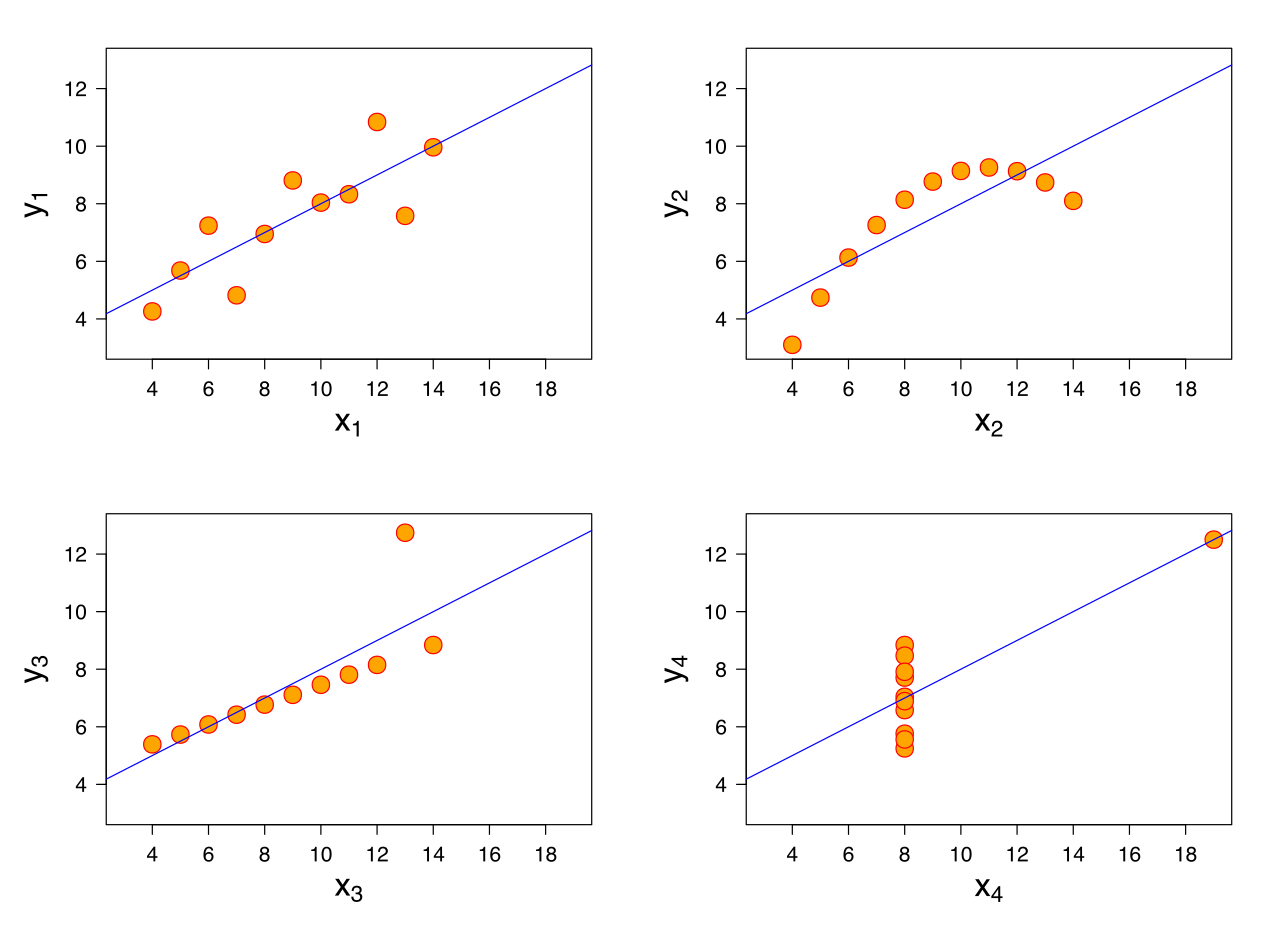
2. r is not resistant. Because it is built from means and squared deviations, a single distant point can drag r dramatically up or down. This is the lesson of Anscombe's quartet in the figure above: four data sets that share essentially the same means, the same r, and the same regression line, yet look nothing alike — one is genuinely linear, one is a clean curve, one is a perfect line ruined by a single outlier, and one is a vertical stack plus one lone point that manufactures the entire correlation.
3. A restricted range shrinks r. If you compute the correlation between admission test scores and college grades using only the students who were admitted, you have thrown away the entire low end of the x range. Cutting the range of x mechanically reduces r, which is why selective samples routinely make good predictors look useless.
4. Correlation is not causation. This is the one everyone can recite and almost no one applies. A strong r between two variables is consistent with at least four different worlds: x causes y; y causes x; a third lurking variable causes both; or the pattern is coincidence in a small sample. Ice cream sales correlate with drowning deaths — because hot weather drives both. The correlation is real; the causal story is fiction. Only a randomized experiment, which breaks the link between the treatment and every lurking variable at once, licenses a causal claim from data like these.
Two smaller notes worth keeping. r requires both variables to be quantitative — there is no correlation between eye color and height. And r is symmetric: the correlation of x with y equals the correlation of y with x. That symmetry is a warning in itself, because it means r alone can never tell you which variable is doing the explaining.
| Value of r | What it says | What it does not say |
|---|---|---|
| r = +1 | Every point on one upward straight line | Nothing about how steep that line is |
| r = +0.90 | Strong positive linear association | That x causes y |
| r = −0.90 | Strong negative association — exactly as strong as +0.90 | That the relationship is "worse" than a positive one |
| r = 0.05 | Almost no linear tendency | That the variables are unrelated — the form may be curved |
| r = −1.4 | Nothing — this is impossible | — check your arithmetic; r lives in [−1, +1] |
- r measures the direction and strength of a linear relationship and always lies between −1 and +1.
- r = 126 ÷ √(42 × 466) = 0.90 for our study-hours data — strong and positive.
- r has no units, is unchanged by rescaling, and is symmetric in x and y.
- r is not resistant to outliers, is blind to curvature, shrinks under a restricted range, and never establishes causation.
Section 3The regression line
What "least squares" means
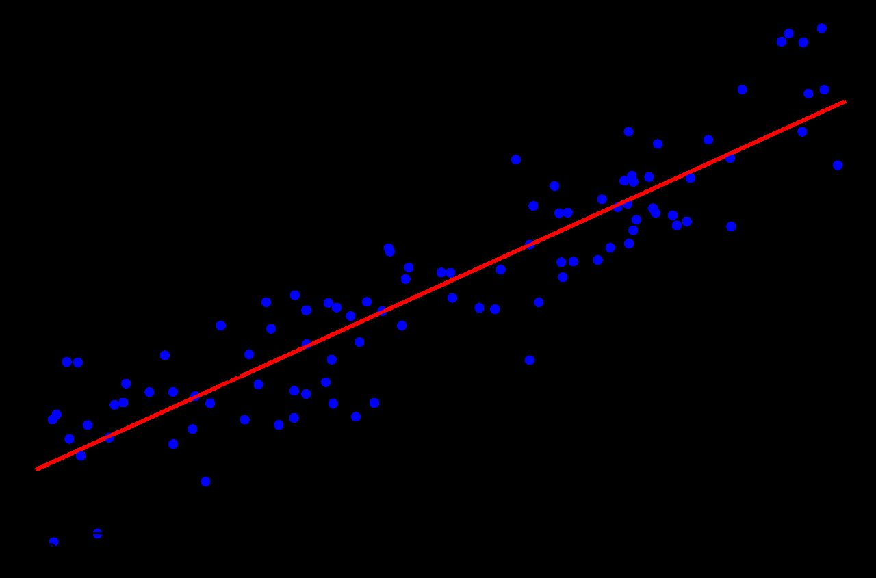
Once a scatterplot looks linear, you can lay a straight line through it and use that line as a model. But infinitely many lines pass through a cloud of points, so we need a rule that picks exactly one. The rule is least squares.
For any candidate line, and for each data point, measure the vertical distance from the point to the line — how far off the line's prediction was. That distance is the residual: residual = y − ŷ, where ŷ ("y-hat") is the value the line predicts. Square every residual so that misses above and below both count as errors and cannot cancel, then add them up. The least-squares regression line is the unique line that makes that sum, Σ(y − ŷ)2, as small as it can possibly be.
Two details in that definition are load-bearing. First, the distances are vertical, not perpendicular — because we are in the business of predicting y from x, and vertical distance is exactly the error in predicting y. Second, we square rather than take absolute values, which has the side effect of making a large miss count disproportionately. That is why one outlier can tilt a regression line so effectively.
An immediate consequence of squaring vertical distances: the regression line of y on x is not the same as the line of x on y. Correlation is symmetric; regression is not. Swap the roles of the variables and you get a different line, so decide which variable you are predicting before you fit anything.
Slope and intercept
Write the line in the familiar form ŷ = a + bx, where b is the slope and a the y-intercept. The least-squares solution is remarkably tidy:
b = Σ(x−x̄)(y−ȳ) ÷ Σ(x−x̄)2 — equivalently b = r × (sy ÷ sx)
a = ȳ − b x̄
The second slope formula is worth staring at. The slope is the correlation, converted from standardized units back into real ones by the ratio of the two standard deviations. It also tells you that the slope and r always share a sign: a positive correlation guarantees an upward line. And the intercept formula is a rearrangement of ȳ = a + bx̄, which says something useful in its own right: the least-squares line always passes through the point of averages (x̄, ȳ). If your line misses that point, you have made an arithmetic error.
Fitting the line to our data
Everything we need is already in the Section 2 table. The slope:
b = 126 ÷ 42 = 3
Check it the other way: b = r × sy ÷ sx = 0.9006 × (9.654 ÷ 2.898) = 0.9006 × 3.331 = 3.00. Agreed. Now the intercept:
a = ȳ − bx̄ = 78 − (3)(6) = 78 − 18 = 60
The least-squares line is ŷ = 60 + 3x. Verify the point of averages: at x = 6, ŷ = 60 + 18 = 78 = ȳ. Correct.
Interpreting the slope. The slope is a rate, and its units are the units of y per unit of x: 3 exam points per hour of study. State it as a prediction, not a promise: "for each additional hour studied, the model predicts an increase of about 3 points in exam score, on average." Not "an extra hour raises your score by 3 points" — that is a causal claim, and this is observational data, so a lurking variable such as prior preparation could be producing both.
Interpreting the intercept. The intercept is the predicted y when x = 0: a student who studies 0 hours is predicted to score 60. Sometimes that is meaningful, sometimes it is nonsense, and the deciding question is always whether x = 0 is inside the range of the data we actually observed. Our hours ran from 2 to 10, so x = 0 sits outside the data — close by, but outside. Treat that 60 as an anchor that positions the line, not as a real forecast about a student who never opens the book.
Proving the line is best
"Least squares" is a claim we can test with arithmetic. Our line gives the following predictions and errors: at x = 2, ŷ = 66 and the actual score was 72, an error of +6; at x = 4, ŷ = 72 versus 69, error −3; at x = 5, ŷ = 75 versus 70, error −5; at x = 7, ŷ = 81 versus 80, error −1; at x = 8, ŷ = 84 versus 83, error −1; at x = 10, ŷ = 90 versus 94, error +4. Squaring and adding: 36 + 9 + 25 + 1 + 1 + 16 = 88.
Now try a steeper line. Keep it through the point of averages — for any slope you fix, the intercept that minimizes the squared errors is a = ȳ − b x̄, so the best line at that slope always passes through (x̄, ȳ) — with slope 3.5, so a = 78 − 3.5(6) = 57 and ŷ = 57 + 3.5x. Its errors are +8, −2, −4.5, −1.5, −2, +2, and the squared total is 64 + 4 + 20.25 + 2.25 + 4 + 4 = 98.5. Worse. A shallower slope of 2.5 gives a = 63, errors +4, −4, −5.5, −0.5, 0, +6, and a squared total of 16 + 16 + 30.25 + 0.25 + 0 + 36 = 98.5. Also worse, and by exactly the same amount — the penalty for missing the best slope is symmetric.
| Candidate line | Slope | Intercept | Σ(y − ŷ)2 | Verdict |
|---|---|---|---|---|
| ŷ = 63 + 2.5x | 2.5 | 63 | 98.5 | Too shallow |
| ŷ = 60 + 3x | 3 | 60 | 88 | Least squares — the best line |
| ŷ = 57 + 3.5x | 3.5 | 57 | 98.5 | Too steep |
No other slope beats 88. That number has a name we will use throughout Section 4: the sum of squared errors, SSE.
- The least-squares line minimizes Σ(y − ŷ)2, the sum of squared vertical distances.
- b = Σ(x−x̄)(y−ȳ) ÷ Σ(x−x̄)2 = r sy ÷ sx; and a = ȳ − b x̄.
- Our line is ŷ = 60 + 3x: predicted score rises about 3 points per extra study hour.
- The line always passes through (x̄, ȳ), and the slope always shares the sign of r.
- Regression is not symmetric — predicting x from y gives a different line.
Section 4r-squared and residuals
Residuals: what the line missed
A residual is the leftover: residual = observed − predicted = y − ŷ. A positive residual means the actual value sat above the line — the individual did better than the model expected. A negative residual means it sat below. The residuals are the raw material for everything in this section, so compute them carefully.
| x (hours) | y (actual) | ŷ = 60 + 3x | Residual y − ŷ | Residual2 |
|---|---|---|---|---|
| 2 | 72 | 66 | +6 | 36 |
| 4 | 69 | 72 | −3 | 9 |
| 5 | 70 | 75 | −5 | 25 |
| 7 | 80 | 81 | −1 | 1 |
| 8 | 83 | 84 | −1 | 1 |
| 10 | 94 | 90 | +4 | 16 |
| Sums | — | — | 0 | 88 |
The residuals sum to exactly zero. That is not luck — it is a mathematical guarantee of least squares, and therefore a free error check every time you do this by hand. Student A, who studied 2 hours and scored 72, has the largest residual: +6 points better than the model predicted. Student C, at 5 hours and 70 points, came in 5 points short.
r2: how much variation the line explains
Before we had a line, our only guess for any student's score would have been the overall mean, 78. The total variation in y around that mean is the total sum of squares, SST = Σ(y − ȳ)2 = 466, which we already computed in Section 2. After fitting the line, the variation still left over is SSE = Σ(y − ŷ)2 = 88. The line therefore accounted for 466 − 88 = 378 of the original variation.
The coefficient of determination is that accounted-for share:
r2 = 1 − (SSE ÷ SST) = 1 − (88 ÷ 466) = 1 − 0.1888 = 0.8112
And it lives up to its name: it really is the square of the correlation. From Section 2, r = 0.9006, and 0.90062 = 0.8111 — the same value up to rounding. So we report r2 = 0.81, or 81%.
The correct sentence is: about 81% of the variation in exam scores is explained by the linear relationship with hours studied. The remaining 19% is variation the line does not capture — sleep, prior knowledge, test anxiety, luck. Three phrasings that sound similar and are all wrong: it does not mean 81% of the points lie on the line; it does not mean predictions are 81% accurate; and it does not mean studying causes 81% of exam performance. r2 is a statement about variation, nothing else.
Because it is a square, r2 always falls between 0 and 1 and is always positive — which means it discards the direction of the relationship. Report r alongside it, or your reader cannot tell whether the association was positive or negative.
Reading a residual plot
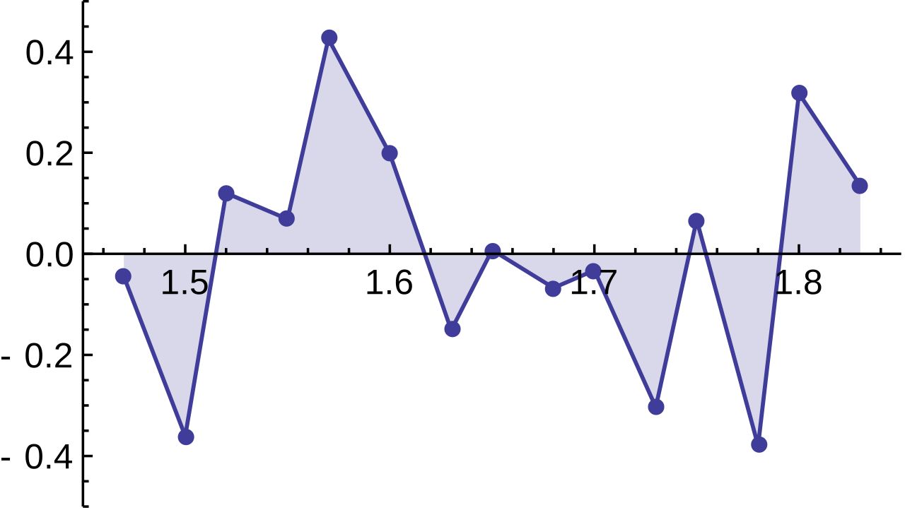
A residual plot graphs the residuals on the vertical axis against x (or against ŷ) on the horizontal. Its whole purpose is to magnify what the original scatterplot hides. In the original plot, a gentle curve can be swamped by the steep overall rise; subtracting the line removes that rise and leaves the misfit standing alone.
What you want to see is nothing: a formless horizontal band of points scattered above and below the zero line, with no shape and roughly constant width. That is the residual plot's way of saying the straight-line model is adequate. Any structure is a message.
| What the residual plot shows | What it means | What to do |
|---|---|---|
| Formless horizontal band around zero | A line is an adequate model | Proceed — report slope, r, r2 |
| A clear U or arch (curvature) | The true form is curved, not linear | Do not use the line; transform a variable or fit a curve |
| A fan widening left to right | Spread of y grows with x (non-constant variance) | Predictions are far less reliable at the wide end |
| One point far from the rest vertically | An outlier in the y direction | Investigate it; report results with and without it |
| One point far out in x with a small residual | A high-leverage, possibly influential point | Refit without it — if the line moves a lot, say so |
Our six residuals, in x order, run +6, −3, −5, −1, −1, +4. They start high, dip negative in the middle, and come back up — a faint U. With only six points that is far too little evidence to abandon the linear model, but it is exactly the pattern you would flag and watch if you collected forty students instead of six.
The distinction in the last two table rows deserves emphasis. Leverage is about being extreme in x; a point far to the right or left of the other x values sits at the end of a long lever and can swing the line. Influence is about actually changing the answer: a point is influential if removing it noticeably moves the slope, the intercept, or r. High-leverage points are the ones most likely to become influential, but the only way to know is to refit without the point and compare.
- Residual = observed − predicted = y − ŷ; residuals from a least-squares line always sum to 0.
- SST = 466 (variation about ȳ), SSE = 88 (variation left after the line), so r2 = 1 − 88÷466 = 0.81.
- Say it as: "81% of the variation in y is explained by the linear relationship with x" — not 81% of points, not 81% accurate, not 81% caused.
- r2 is always positive, so it hides direction — report r too.
- A good residual plot shows no pattern; curvature, fanning, or a lone stray point each mean something different.
Section 5Prediction
Using the line
Prediction is mechanical: put a value of x into the equation and read off ŷ. With ŷ = 60 + 3x, a student who studies 6 hours is predicted to score 60 + 3(6) = 78; a student who studies 9 hours is predicted to score 60 + 3(9) = 87.
What is not mechanical is knowing what that number means. The regression line predicts the average y for individuals with that x, not the value any one individual will get. Our own data prove the point: student E studied 8 hours, the line predicted 84, and the actual score was 83. Off by one. Student A studied 2 hours, the line predicted 66, and the actual was 72 — off by six. A prediction from a regression line is a center of gravity, not a guarantee.
You can quantify the typical miss. The standard error of the estimate measures the typical size of a residual:
se = √[ SSE ÷ (n − 2) ] = √(88 ÷ 4) = √22 = 4.69 points
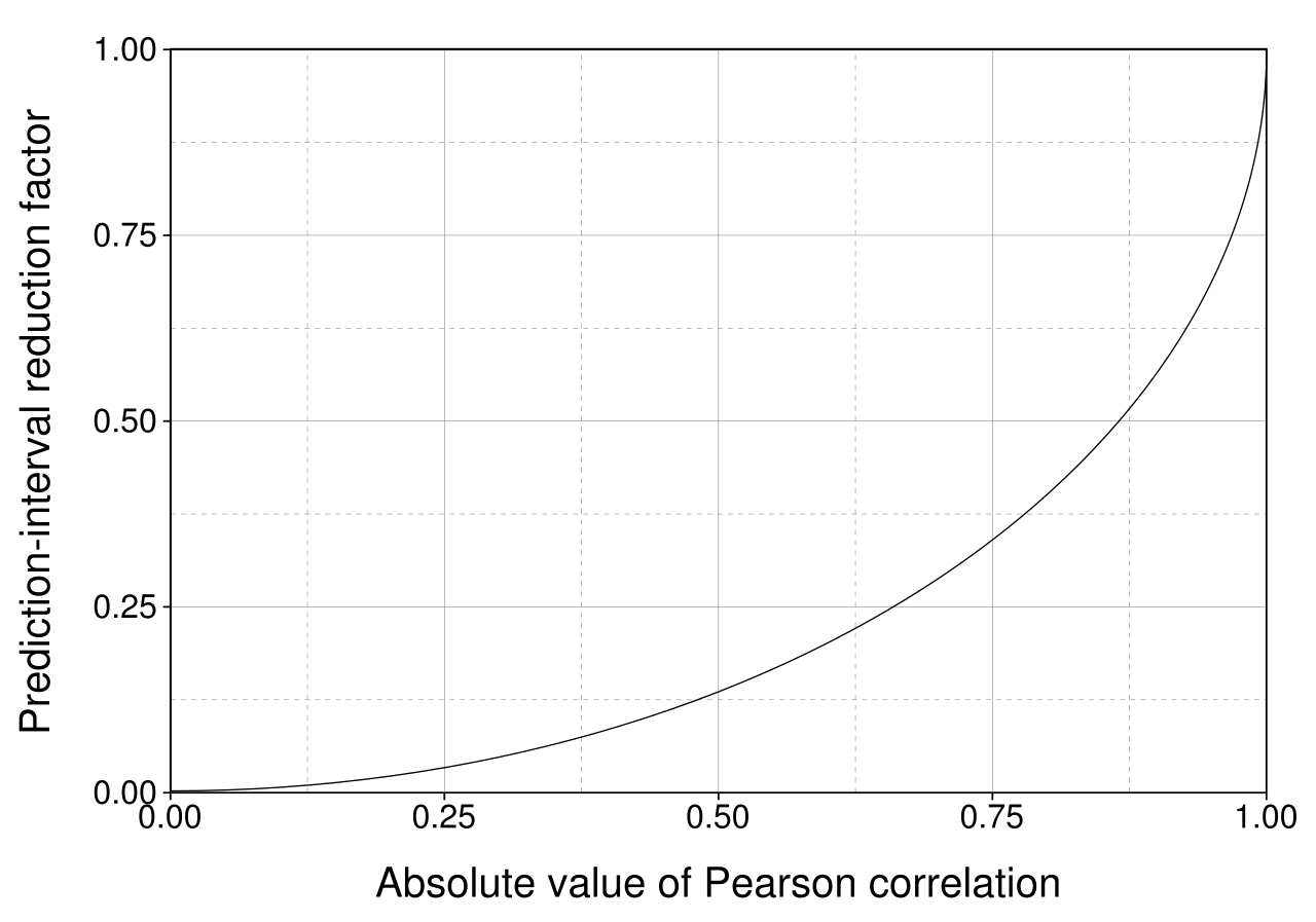
We divide by n − 2 rather than n − 1 because fitting a line consumed two pieces of information — a slope and an intercept. Interpretation: individual scores fall about 4.7 points away from the regression line, on average. So the prediction of 87 for a nine-hour student is better read as "somewhere in the mid-to-high 80s, give or take five points or so," and a rough working range of ŷ ± 2se — roughly 78 to 96 — is a serviceable ballpark. It is only a ballpark: a proper prediction interval is wider than that near the edges of the data, which is exactly the flaring you see in the figure above.
Interpolation is safe; extrapolation is not
Interpolation means predicting at an x value inside the range you observed. Our hours ran from 2 to 10, so predicting for 6 hours is interpolation, and it rests on evidence: we watched what happened to students on both sides of 6.
Extrapolation means predicting outside that range, and it rests on an assumption you cannot check — that the straight-line pattern continues where you have no data. Very often it does not. Watch what our perfectly reasonable line does when pushed:
| Hours (x) | Prediction ŷ = 60 + 3x | Inside the data (2–10)? | Verdict |
|---|---|---|---|
| 3 | 69 | Yes | Interpolation — trustworthy |
| 6 | 78 | Yes | Interpolation — trustworthy |
| 9 | 87 | Yes | Interpolation — trustworthy |
| 0 | 60 | No (just outside) | The intercept — anchors the line, not a real forecast |
| 15 | 105 | No | Impossible — the exam is out of 100 |
| 25 | 135 | No | Absurd — the model has left reality behind |
The line never warns you. It will happily return 135 for a 25-hour student, because a line is an infinite object and arithmetic has no common sense. The real relationship must flatten — scores are capped at 100, and past some point extra hours yield nothing or actively hurt through fatigue. Our data simply never visited that region, so our line knows nothing about it. Always state the range of x your model was built on, and refuse predictions outside it.
Four more habits before you predict
Do not predict backwards with the same line. Our line predicts score from hours. To predict hours from score you must refit with the roles reversed — that line has slope 126 ÷ 466 = 0.27, not 1 ÷ 3. Algebraically inverting a regression line gives the wrong answer.
Remember regression to the mean. Because the slope is r × sy ÷ sx and r is less than 1 in size, predictions are always pulled toward ȳ relative to how extreme x was. A student one full standard deviation above average in hours is predicted only r = 0.90 standard deviations above average in score. This is not a defect; it is a consequence of imperfect correlation, and it explains why exceptional performances tend to be followed by more ordinary ones without any cause at all.
Check the conditions before you trust any inference. The descriptive tools — r, the slope, r2 — only need a roughly linear scatterplot. But the moment you attach a p-value or a confidence interval to the slope, you are relying on a model, and that model has four stated assumptions. Linearity: the true relationship between x and y is a straight line — check the scatterplot and confirm with a patternless residual plot. Independence: the observations are independent of one another, which comes from how the data were collected, not from anything you can see in a plot. Constant variance: the spread of y about the line is the same across the range of x — the fanning row in the Section 4 table is exactly this condition failing. Approximate Normality: the residuals are roughly Normal about the line, checked with a histogram or Normal plot of the residuals. Our six students are far too few to check any of this convincingly, which is itself the honest report.
Be precise about uncertainty language. Regression output usually includes a test of whether the slope differs from zero, along with a p-value and a confidence interval. Three statements must be kept straight. First, a p-value is the probability of getting data at least this extreme if the true slope were zero — it is not the probability that the true slope is zero, and not the probability that your finding is wrong. Second, a large p-value means you fail to reject the hypothesis of zero slope; it does not let you accept that the slope is zero. Absence of evidence for a relationship is not evidence that there is none — a small sample can hide a real slope easily. Third, a 95% confidence interval for the slope describes the long-run behavior of the procedure: if you repeated the whole study many times, about 95% of the intervals constructed this way would contain the true slope. It does not mean there is a 95% chance the true slope lies inside the one interval in front of you — that interval either contains it or it does not.
- Substituting x into the line predicts the average y at that x, not any individual's value.
- se = √[SSE ÷ (n−2)] = √22 = 4.69 — the typical distance of a point from the line.
- Interpolation (inside the observed x range) is supported by data; extrapolation is not, and produced an impossible 105 at 15 hours.
- To predict x from y, refit — do not invert the equation.
- Inference about the slope assumes linearity, independence, constant variance, and roughly Normal residuals — state and check them.
- A p-value is not the probability the null is true; failing to reject a zero slope is not accepting it; and a 95% CI describes the long-run procedure, not this one interval.
The chapter in one breath
- A scatterplot shows two quantitative variables on the same individuals; describe it as form, direction, strength, outliers, with the explanatory variable on the x-axis.
- r measures the direction and strength of a linear relationship, lies in [−1, +1], has no units, and is symmetric; for our data r = 126 ÷ √(42×466) = 0.90.
- r is blind to curvature, vulnerable to outliers, shrunk by a restricted range, and silent about causation — a lurking variable can produce any correlation you like.
- The least-squares line minimizes Σ(y−ŷ)2; b = r sy÷sx = 3 and a = ȳ − b x̄ = 60, giving ŷ = 60 + 3x, which passes through (6, 78).
- The slope is a predicted rate of change (3 points per hour); the intercept is only meaningful if x = 0 sits within the data.
- Residuals (y − ŷ) sum to zero and give SSE = 88; with SST = 466, r2 = 0.81 — 81% of the variation in scores is explained by the linear relationship with hours.
- A residual plot should look like nothing at all; curvature, fanning, and stray points each diagnose a different failure that r2 alone would hide.
- Interpolate freely, never extrapolate — our line predicts an impossible 105 at 15 hours — and report every prediction with its typical error se = 4.69 and its range of validity.
- Inference on the slope assumes linearity, independence, constant variance, and roughly Normal residuals; a p-value is not the probability the null is true, failing to reject is not accepting, and a 95% CI is a claim about the procedure.
ReferenceWords worth knowing
A quick reference for the terms in this chapter — skim it now, or circle back whenever a word trips you up.
- Coefficient of determination (r2)
- The proportion of the variation in y explained by the linear relationship with x; equals 1 − SSE÷SST, and equals the square of r.
- Correlation coefficient (r)
- A unit-free number between −1 and +1 measuring the direction and strength of a straight-line relationship between two quantitative variables.
- Explanatory variable
- The variable used to explain or predict the other; plotted on the horizontal axis and denoted x. Also called the predictor or independent variable.
- Extrapolation
- Predicting at an x value outside the range of the observed data; unsupported by evidence and a common source of absurd results.
- Fitted value (ŷ)
- The value the regression line predicts for a given x; also called the predicted value.
- Influential point
- An observation whose removal noticeably changes the slope, intercept, or r. Usually a high-leverage point — one extreme in the x direction, sitting at the end of a long lever — but only refitting without it can confirm influence.
- Intercept (a)
- The predicted value of y when x = 0; computed as ȳ − b x̄ and meaningful only if x = 0 falls within the data.
- Interpolation
- Predicting at an x value inside the observed range; the legitimate use of a regression line.
- Least-squares regression line
- The unique line ŷ = a + bx that makes the sum of squared vertical distances from the points to the line as small as possible.
- Lurking variable
- A third variable, not measured, that affects both x and y and can create a correlation with no causal link between them.
- Outlier
- A point lying far from the overall pattern of the scatterplot; it need not be extreme on either variable alone.
- Regression to the mean
- The tendency for predicted y values to be less extreme than their x values, because the slope is r times sy÷sx and |r| is less than 1.
- Residual
- Observed minus predicted, y − ŷ; positive above the line, negative below, and always summing to zero for a least-squares fit.
- Residual plot
- A graph of residuals against x (or against ŷ); a good one shows no pattern at all.
- Response variable
- The outcome being explained or predicted; plotted on the vertical axis and denoted y. Also called the dependent variable.
- Restricted range
- A sample that covers only part of the possible x values, which mechanically shrinks r and hides a real relationship.
- Scatterplot
- A graph of two quantitative variables measured on the same individuals, one dot per individual.
- Slope (b)
- The predicted change in y for a one-unit increase in x; equals r × sy ÷ sx and always shares the sign of r.
- Spurious correlation
- A strong association between variables that have no causal connection, typically produced by a lurking variable or by chance.
- Standard error of the estimate (se)
- The typical size of a residual, √[SSE ÷ (n − 2)]; a root-mean-square measure of how far observed points fall from the line, divided by n − 2 because the fit consumed a slope and an intercept.
- Sum of squared errors (SSE)
- Σ(y − ŷ)2, the variation in y left unexplained after fitting the line.
- Total sum of squares (SST)
- Σ(y − ȳ)2, the total variation in y about its mean before any line is fitted.