Polynomial & Rational Functions
Up to now most of the functions you have graphed have been lines and parabolas — one bend at most. This chapter opens the door to curves with several bends, curves that shoot off to infinity, and curves with invisible walls they can never cross. The good news is that you do not have to plot a hundred points to draw any of them. A polynomial's whole personality is written in two numbers — its degree and its leading coefficient — and a rational function's whole personality falls out of one move: factor the top, factor the bottom, and see what cancels. Everything in this chapter is a checklist, and we will walk every checklist one slow step at a time.
By the end of this chapter you can
- Recognize a polynomial function and state its degree and leading coefficient.
- Predict a polynomial's end behavior from degree and leading coefficient alone.
- Find the zeros of a polynomial by factoring and using the zero-product property.
- Use multiplicity to decide whether a graph crosses the x-axis or touches and turns around.
- Divide polynomials by long division and by synthetic division.
- Apply the Remainder Theorem and Factor Theorem to test and peel off factors.
- State the domain of a rational function and locate its vertical asymptotes, horizontal asymptotes, and holes.
- Assemble a complete, correct sketch of a rational function from its intercepts, asymptotes, and sign chart.
Section 1Polynomial graphs: degree, leading coefficient, and end behavior
What makes a function a polynomial
A polynomial function is a sum of terms, each one a number multiplied by x raised to a whole-number power. Written out in full it looks like this:
P(x) = anxn + an−1xn−1 + … + a1x + a0, with an ≠ 0
That looks intimidating, so translate it. The exponents must be 0, 1, 2, 3, … — never negative, never a fraction. The coefficients (the numbers out front) can be anything real. And an ≠ 0 just means we are not allowed to pretend a term is there when its coefficient is zero.
Three quick sorting decisions. f(x) = 4x3 − x + 9 is a polynomial: exponents 3, 1, and 0. g(x) = 5/x + 2 is not, because 5/x is really 5x−1 and negative exponents are banned. h(x) = √x + 1 is not, because √x is x1/2 and fractional exponents are banned too. Those two outlaws are not useless — the first one is a rational function and shows up later in this very chapter — they simply are not polynomials.
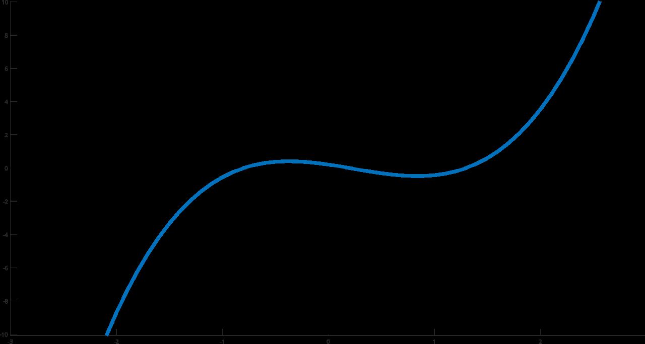
Two visual consequences follow immediately, and they are worth memorizing because they are what let you sketch quickly. A polynomial graph is continuous (you can draw it without lifting your pencil — no gaps, no jumps) and smooth (no sharp corners, only gentle turns).
Degree and leading coefficient
Write the polynomial in standard form — highest exponent first, descending down to the constant. Then the degree is that highest exponent, and the leading coefficient is the number sitting in front of it. Order matters here only because it is easy to grab the wrong term from a jumbled expression; rearranging first costs you five seconds and saves you the mistake.
Consider f(x) = 4x − 2x3 + 5x2 − 1. Rearranged: f(x) = −2x3 + 5x2 + 4x − 1. Now it is obvious: degree 3, leading coefficient −2. Notice the leading coefficient carries its sign with it. It is −2, not 2, and that minus sign is about to decide which way the whole graph points.
The degree also caps two counts. A degree-n polynomial has at most n real zeros (x-intercepts) and at most n − 1 turning points — places where the curve stops rising and starts falling, or vice versa. A cubic can wiggle twice; it can never wiggle three times.
End behavior: what the graph does at the far edges
End behavior answers a simple question: if you follow the curve far to the right and far to the left, does each arm go up or down? Out at the extremes, the highest-power term completely dominates every other term, so only two facts matter — whether the degree is even or odd, and whether the leading coefficient is positive or negative. Four combinations, four pictures.
| Degree | Leading coefficient | Left end (as x → −∞) | Right end (as x → +∞) | Looks like |
|---|---|---|---|---|
| Even | Positive | Rises (→ +∞) | Rises (→ +∞) | Both arms up, like y = x2 |
| Even | Negative | Falls (→ −∞) | Falls (→ −∞) | Both arms down, like y = −x2 |
| Odd | Positive | Falls (→ −∞) | Rises (→ +∞) | Down-left, up-right, like y = x3 |
| Odd | Negative | Rises (→ +∞) | Falls (→ −∞) | Up-left, down-right, like y = −x3 |
If the table feels like four things to memorize, it is really only two. Even degree means the two ends agree (both up or both down, like a parabola). Odd degree means the two ends disagree (one up, one down). Then a negative leading coefficient simply flips whatever picture you just drew upside down.
Worked example — every step
Describe the end behavior of f(x) = −2x3 + 5x2 + 4x − 1, then prove it with actual arithmetic.
Step 1 — find the degree. The exponents present are 3, 2, 1, and 0. The highest is 3, so the degree is 3. Three is odd.
Step 2 — find the leading coefficient. The degree-3 term is −2x3, so the leading coefficient is −2. That is negative.
Step 3 — read the table. Odd degree with a negative leading coefficient: the graph rises on the left and falls on the right.
Step 4 — check the right end with a real number. Substitute x = 10 and do each piece separately:
- −2(10)3 = −2(1000) = −2000
- 5(10)2 = 5(100) = 500
- 4(10) = 40
- the constant is −1
Add them in order: −2000 + 500 = −1500; then −1500 + 40 = −1460; then −1460 − 1 = −1461. So f(10) = −1461 — a big negative number. The right arm is heading down. That matches Step 3.
Step 5 — check the left end. Substitute x = −10. Watch the signs carefully, because this is where most errors happen:
- −2(−10)3 = −2(−1000) = +2000 (an odd power of a negative number is negative, and the leading −2 flips it back to positive)
- 5(−10)2 = 5(100) = 500 (an even power of a negative number is positive)
- 4(−10) = −40
- the constant is −1
Add in order: 2000 + 500 = 2500; then 2500 − 40 = 2460; then 2460 − 1 = 2459. So f(−10) = 2459 — a big positive number. The left arm is heading up. Step 3 confirmed from both directions.
Step 6 — bound the wiggles. Degree 3 means at most 3 x-intercepts and at most 3 − 1 = 2 turning points. So the sketch is: come down from the upper left (Step 5 gave f(−10) = 2459, high above the axis), wiggle at most twice, and leave toward the lower right (Step 4 gave f(10) = −1461, far below it).
- A polynomial allows only whole-number exponents; its graph is continuous and smooth.
- Degree = highest exponent; leading coefficient = the number in front of it (sign included).
- Even degree → both ends agree; odd degree → the ends disagree; a negative leading coefficient flips the picture.
- Degree n allows at most n real zeros and at most n − 1 turning points.
Section 2Zeros and multiplicity
Four words for the same thing
A zero of P(x) is any number c with P(c) = 0. Textbooks and instructors will also call it a root of the equation P(x) = 0, a solution of that equation, or an x-intercept of the graph. These are four names for one idea, viewed from four angles: function language, equation language, solving language, and graph language. If c is a real zero, the point (c, 0) is on the graph.
The engine that finds zeros is the zero-product property: if a product of factors equals zero, then at least one of those factors is zero. So the strategy never changes — factor the polynomial completely, then set each factor equal to zero and solve. The strategy is easy; the factoring is the work.
One theorem makes the connection official. The Factor Theorem says (x − c) is a factor of P(x) exactly when P(c) = 0. Factors and zeros are two views of the same fact, and Section 3 turns that into a practical tool.
Worked example — finding zeros by factoring
Find all real zeros of P(x) = x3 + 2x2 − 8x.
Step 1 — pull out the greatest common factor. Every term contains at least one x, so factor x out: P(x) = x(x2 + 2x − 8). Never skip this step — students who jump straight to the quadratic formula routinely lose the zero at x = 0.
Step 2 — factor the trinomial. For x2 + 2x − 8 we need two numbers that multiply to −8 and add to +2. Test the pairs: 1 and −8 add to −7 (no); −1 and 8 add to 7 (no); 2 and −4 add to −2 (no); −2 and 4 add to +2 (yes). So x2 + 2x − 8 = (x + 4)(x − 2), and the whole thing is P(x) = x(x + 4)(x − 2).
Step 3 — set each factor to zero. x = 0 gives x = 0. Then x + 4 = 0 gives x = −4. Then x − 2 = 0 gives x = 2.
Step 4 — check every answer by substituting. This is the step that catches sign errors, and it takes fifteen seconds.
- P(0) = 03 + 2(0)2 − 8(0) = 0 + 0 − 0 = 0 ✓
- P(−4) = (−4)3 + 2(−4)2 − 8(−4) = −64 + 2(16) + 32 = −64 + 32 + 32 = 0 ✓
- P(2) = 23 + 2(2)2 − 8(2) = 8 + 2(4) − 16 = 8 + 8 − 16 = 0 ✓
The zeros are x = −4, x = 0, and x = 2, so the graph crosses the horizontal axis at (−4, 0), (0, 0), and (2, 0). Degree 3 allowed at most three, and we found three.
Multiplicity: cross, or touch and turn
Sometimes a factor repeats. In Q(x) = (x − 5)2(x + 1), the factor (x − 5) appears twice. The exponent on a factor is called the multiplicity of that zero: 5 is a zero of multiplicity 2, and −1 is a zero of multiplicity 1. Multiplicity is not bookkeeping trivia. It tells you exactly what the curve does when it arrives at that point on the axis.
| Multiplicity | Example factor | What the graph does there | Does the sign of P(x) change? |
|---|---|---|---|
| 1 (odd) | (x − 2) | Passes straight through the axis | Yes |
| 2 (even) | (x − 2)2 | Touches the axis and turns back — a bounce | No |
| 3 (odd) | (x − 2)3 | Crosses, but flattens out on the way through | Yes |
| 4 (even) | (x − 2)4 | Touches, flattens hard, and turns back | No |
| Any odd | — | Cross | Yes |
| Any even | — | Touch and turn | No |
Here is the reason, in one line. Near x = 2 the factor (x − 2) is negative on the left and positive on the right. Raise a quantity that changes sign to an even power and the result is positive on both sides — no sign change, so the graph stays on one side of the axis and must turn around. Raise it to an odd power and the sign survives — negative becomes positive, so the graph passes through.
Multiplicities also account for the degree. Add up all the multiplicities and you get the degree of the polynomial. In f(x) = (x + 2)(x − 1)2(x − 3)3 the multiplicities are 1, 2, and 3, so the degree is 1 + 2 + 3 = 6.
Worked example — a full sketch from factors
Describe the graph of f(x) = (x + 2)(x − 1)2(x − 3)3.
Step 1 — list zeros with multiplicities. Set each factor to zero. x + 2 = 0 → x = −2, multiplicity 1. x − 1 = 0 → x = 1, multiplicity 2. x − 3 = 0 → x = 3, multiplicity 3.
Step 2 — degree. 1 + 2 + 3 = 6. The degree is 6, which is even.
Step 3 — leading coefficient. Multiplying out would take a while, but we only need the leading term. Each factor contributes its own x: (x)(x)2(x)3 = x6, with coefficient 1 · 1 · 1 = 1. The leading coefficient is +1, positive.
Step 4 — end behavior. Even degree, positive leading coefficient → both ends rise.
Step 5 — behavior at each zero. At x = −2 (multiplicity 1, odd) the graph crosses plainly. At x = 1 (multiplicity 2, even) it touches and turns around without crossing. At x = 3 (multiplicity 3, odd) it crosses, flattening as it goes through.
Step 6 — the y-intercept, with the arithmetic shown. Substitute x = 0: f(0) = (0 + 2)(0 − 1)2(0 − 3)3 = (2)(−1)2(−3)3. Now (−1)2 = 1 and (−3)3 = −27, so f(0) = (2)(1)(−27) = −54. The graph passes through (0, −54).
Step 7 — assemble it. Coming down from the upper left, the curve crosses at x = −2 into negative territory, dips through (0, −54), rises to just touch the axis at x = 1 and bounce back down, then crosses upward at x = 3 with a flat spot, and rises forever. That is a complete, correct shape and we never plotted a table of points.
- Zero, root, solution, x-intercept all name the same number viewed four ways.
- Factor completely, then apply the zero-product property — and always check answers by substituting back.
- Odd multiplicity → the graph crosses; even multiplicity → it touches and turns around.
- The multiplicities add up to the degree, and the leading coefficient can be read off the factors without expanding.
Section 3Dividing polynomials
Why divide at all
Factoring a cubic or quartic by inspection is often hopeless. Division rescues you: if you can find one zero, dividing by its factor drops the degree by one, and you keep dropping until what is left is a quadratic you can factor or run through the quadratic formula. Division is also the only clean way to find the slant asymptote of a rational function, which is waiting for you in Section 5.
The bookkeeping is identical to the long division you learned with whole numbers. Dividing 17 by 5 gives a quotient of 3 and a remainder of 2, and we can write 17 = 5 · 3 + 2. Polynomials obey the same identity:
dividend = divisor · quotient + remainder, or P(x) = D(x) · Q(x) + R(x), where the degree of R(x) is less than the degree of D(x).
That identity is your answer-checker. Multiply the divisor by the quotient, add the remainder, and you must get the original polynomial back. If you do not, something went wrong and you now know it before you turn the page.
Worked example — long division, one step at a time
Divide x3 − 4x2 + 2x + 5 by x − 3.
Step 1 — divide the leading terms. x3 ÷ x = x2. Write x2 as the first term of the quotient. Multiply it back through the divisor: x2(x − 3) = x3 − 3x2. Subtract that from the first two terms of the dividend: (x3 − 4x2) − (x3 − 3x2) = x3 − x3 − 4x2 + 3x2 = −x2. Bring down the +2x, giving −x2 + 2x.
Step 2 — repeat. −x2 ÷ x = −x. That is the next quotient term. Multiply back: −x(x − 3) = −x2 + 3x. Subtract: (−x2 + 2x) − (−x2 + 3x) = −x2 + x2 + 2x − 3x = −x. Bring down the +5, giving −x + 5.
Step 3 — repeat once more. −x ÷ x = −1. Multiply back: −1(x − 3) = −x + 3. Subtract: (−x + 5) − (−x + 3) = −x + x + 5 − 3 = 2.
Step 4 — stop and read off the answer. The leftover 2 has degree 0, which is less than the divisor's degree 1, so we stop. The quotient is x2 − x − 1 and the remainder is 2:
(x3 − 4x2 + 2x + 5)/(x − 3) = x2 − x − 1 + (2)/(x − 3)
Step 5 — check it. Multiply divisor by quotient: (x − 3)(x2 − x − 1). Distribute the x: x3 − x2 − x. Distribute the −3: −3x2 + 3x + 3. Combine: x3 + (−x2 − 3x2) + (−x + 3x) + 3 = x3 − 4x2 + 2x + 3. Now add the remainder 2: x3 − 4x2 + 2x + 5. That is the original dividend exactly. ✓
Synthetic division: the shortcut for x − c
When — and only when — the divisor has the form x − c, you can throw away the letters and work with the coefficients alone. That is synthetic division. Two setup rules make or break it: use c from the form x − c (so dividing by x + 2 means c = −2), and write a 0 placeholder for every missing power.
Redo the same division, x3 − 4x2 + 2x + 5 divided by x − 3, synthetically. Coefficients: 1, −4, 2, 5. Divisor x − 3 means c = 3.
Step 1. Bring the first coefficient straight down: 1.
Step 2. Multiply it by c: 1 × 3 = 3. Add to the next coefficient: −4 + 3 = −1.
Step 3. Multiply: −1 × 3 = −3. Add to the next coefficient: 2 + (−3) = −1.
Step 4. Multiply: −1 × 3 = −3. Add to the last coefficient: 5 + (−3) = 2.
The bottom row reads 1, −1, −1, and then 2. The last number is always the remainder; the numbers before it are the quotient's coefficients, starting one degree lower than the dividend. The dividend was degree 3, so the quotient is degree 2: x2 − x − 1, remainder 2. Identical to the long-division answer, in about a quarter of the writing.
| Long division | Synthetic division | |
|---|---|---|
| Works for | Any divisor: x − 3, x2 + 1, 3x − 5, anything | Only divisors of the form x − c |
| You write | Full terms with variables | Coefficients only |
| Operations | Divide, multiply, subtract, bring down | Multiply and add (no subtracting) |
| Missing terms | Leave a gap or write 0x2 | Must write a 0 placeholder |
| Speed | Slower, more writing | Fast once the setup is right |
| Typical use | Slant asymptotes, quadratic divisors | Testing candidate zeros, peeling off factors |
The Remainder and Factor Theorems
Two theorems turn division into a zero-finding machine. The Remainder Theorem: when you divide P(x) by x − c, the remainder equals P(c). Check it against the example above: P(3) = 33 − 4(3)2 + 2(3) + 5 = 27 − 4(9) + 6 + 5 = 27 − 36 + 6 + 5 = 2. The remainder was 2. ✓
The Factor Theorem is the special case that matters most: if the remainder is 0, then P(c) = 0, which means c is a zero and (x − c) is a factor. Remainder zero, factor found.
Which numbers should you test? The Rational Zero Theorem narrows the field: any rational zero of a polynomial with integer coefficients must be of the form (factor of the constant term)/(factor of the leading coefficient). It does not promise a zero exists — it just hands you a short list instead of infinitely many numbers.
Worked example — factoring a cubic completely
Factor P(x) = x3 − 4x2 + x + 6 completely and list its zeros.
Step 1 — build the candidate list. The constant term is 6, with factors 1, 2, 3, 6. The leading coefficient is 1, with factor 1. So the candidates are ±1, ±2, ±3, ±6.
Step 2 — test candidates until one works. Try x = 1: P(1) = 1 − 4 + 1 + 6 = 4. Not zero. Try x = −1: P(−1) = (−1)3 − 4(−1)2 + (−1) + 6 = −1 − 4(1) − 1 + 6 = −1 − 4 − 1 + 6 = 0. Zero found. By the Factor Theorem, (x + 1) is a factor.
Step 3 — divide it out synthetically. Coefficients 1, −4, 1, 6; the factor (x + 1) is (x − (−1)), so c = −1.
- Bring down 1.
- 1 × (−1) = −1; then −4 + (−1) = −5.
- −5 × (−1) = 5; then 1 + 5 = 6.
- 6 × (−1) = −6; then 6 + (−6) = 0. The remainder is 0, exactly as promised.
Step 4 — factor what is left. The bottom row 1, −5, 6 means the quotient is x2 − 5x + 6. Two numbers multiplying to 6 and adding to −5 are −2 and −3, so x2 − 5x + 6 = (x − 2)(x − 3).
Step 5 — write the full factorization and the zeros. P(x) = (x + 1)(x − 2)(x − 3), so the zeros are x = −1, x = 2, and x = 3, each with multiplicity 1 — the graph crosses at all three.
Step 6 — check by expanding. First (x − 2)(x − 3) = x2 − 3x − 2x + 6 = x2 − 5x + 6. Then (x + 1)(x2 − 5x + 6) = x3 − 5x2 + 6x + x2 − 5x + 6 = x3 − 4x2 + x + 6. Original recovered. ✓
- dividend = divisor · quotient + remainder — multiply back to check every division.
- Long division handles any divisor; synthetic division is faster but only for x − c.
- Remainder Theorem: dividing by x − c leaves remainder P(c).
- Factor Theorem: remainder 0 means c is a zero and (x − c) is a factor — then factor the smaller quotient.
Section 4Rational functions: domain, asymptotes, and holes
Domain: the first question, always
A rational function is one polynomial divided by another: f(x) = P(x)/Q(x), where Q(x) is not the zero polynomial. Every rule you already know about fractions applies, and the biggest one is that division by zero is undefined. So the domain of a rational function is every real number except those that make the denominator zero.
The procedure is short: set the denominator equal to zero, solve, and exclude those values. For f(x) = (x + 1)/(x − 4), setting x − 4 = 0 gives x = 4, so the domain is all real numbers with x ≠ 4. Notice we never look at the numerator for this. The numerator can be zero all day long — that just produces an x-intercept, which is perfectly legal.
Do this before you simplify. This is the single most important habit in the section, and Section 5's pearl will say it again, because cancelling first destroys the evidence of where the function was undefined.
What happens at an excluded value: hole or wall?
An excluded x-value is a place the graph cannot occupy, but there are two very different ways it can be missing, and factoring tells them apart.
If the offending factor cancels with a matching factor in the numerator, the gap is only one point wide: a hole, also called a removable discontinuity. The curve looks perfectly normal on both sides and you draw a small open circle at the missing point.
If the offending factor survives in the denominator after all cancelling, then near that x-value the denominator shrinks toward zero while the numerator does not, so the quotient blows up. That is a vertical asymptote — an invisible vertical wall the graph races along but never touches or crosses.
To find the height of a hole, substitute the missing x-value into the simplified function. The original will only hand you 0/0.
Worked example — domain, hole, and vertical asymptote
For f(x) = (x2 − 9)/(x2 − x − 6), find the domain, any holes, and any vertical asymptotes.
Step 1 — factor top and bottom. The numerator is a difference of squares: x2 − 9 = (x − 3)(x + 3). For the denominator, find two numbers multiplying to −6 and adding to −1: those are −3 and +2, so x2 − x − 6 = (x − 3)(x + 2). The function is now
f(x) = [(x − 3)(x + 3)]/[(x − 3)(x + 2)]
Step 2 — state the domain right now, before cancelling. The denominator is zero when x − 3 = 0 (so x = 3) or x + 2 = 0 (so x = −2). Domain: all real x with x ≠ 3 and x ≠ −2.
Step 3 — cancel. The factor (x − 3) appears top and bottom, so f(x) = (x + 3)/(x + 2), valid for x ≠ 3. That trailing restriction is not optional decoration — it is the whole record of the hole.
Step 4 — the cancelled factor gives a hole. Because (x − 3) cancelled, there is a hole at x = 3. Its height comes from the simplified form: (3 + 3)/(3 + 2) = 6/5 = 1.2. So the hole sits at the point (3, 6/5).
Step 5 — the surviving factor gives a vertical asymptote. The factor (x + 2) did not cancel, so there is a vertical asymptote at x = −2.
Step 6 — confirm the blow-up numerically. Approach −2 from the right using the simplified form. At x = −1.9: (−1.9 + 3)/(−1.9 + 2) = 1.1/0.1 = 11. At x = −1.99: 1.01/0.01 = 101. At x = −1.999: 1.001/0.001 = 1001. The values are rocketing to +∞. From the left, at x = −2.001: 0.999/(−0.001) = −999 — plunging to −∞. A genuine wall, with the graph going opposite directions on its two sides.
Horizontal asymptotes: a contest between degrees
A horizontal asymptote describes the far-left and far-right behavior: the value the outputs settle toward as x runs off to ±∞. Since Section 1 established that only leading terms matter out there, comparing the two leading terms answers the question. Let n be the degree of the numerator and m the degree of the denominator.
| Comparison | End behavior | Example | Result |
|---|---|---|---|
| n < m | Bottom grows faster, so the fraction shrinks | (4x)/(x2 + 1) | Horizontal asymptote y = 0 |
| n = m | They grow at the same rate | (3x2 + 5)/(x2 − 4) | y = 3/1 = 3 (ratio of leading coefficients) |
| n = m + 1 | Top wins by exactly one degree | (x2 − 3x − 4)/(x − 2) | No horizontal asymptote; a slant asymptote instead |
| n > m + 1 | Top runs away entirely | (x4 + 1)/(x − 1) | No horizontal and no slant asymptote |
Test the equal-degree row with real numbers so the rule stops feeling like a rule. For g(x) = (3x2 + 5)/(x2 − 4) at x = 100: the numerator is 3(10000) + 5 = 30005 and the denominator is 10000 − 4 = 9996, so g(100) = 30005/9996 ≈ 3.0017. At x = 1000: numerator 3,000,005, denominator 999,996, quotient ≈ 3.000017. It is squeezing in on y = 3, exactly as the ratio 3/1 predicted.
When the numerator's degree is exactly one more than the denominator's, divide and read the polynomial part. For (x2 − 3x − 4)/(x − 2), run synthetic division with c = 2 on coefficients 1, −3, −4: bring down 1; 1 × 2 = 2 and −3 + 2 = −1; −1 × 2 = −2 and −4 + (−2) = −6. So the quotient is x − 1 with remainder −6, meaning the function equals x − 1 − 6/(x − 2). As x grows, the fraction 6/(x − 2) fades to nothing and the graph hugs the line y = x − 1. Check it at x = 100: the function gives (10000 − 300 − 4)/98 = 9696/98 ≈ 98.94, while the line gives 100 − 1 = 99. The gap is only 0.06, and it keeps closing.
- A rational function is a polynomial over a polynomial; its domain excludes every zero of the denominator.
- Factor first, and write the domain before cancelling anything.
- A cancelled factor produces a hole (get its height from the simplified form); a surviving denominator factor produces a vertical asymptote.
- Horizontal asymptote by degrees: smaller top → y = 0; equal → ratio of leading coefficients; top bigger by one → slant asymptote.
Section 5Graphing rational functions: putting the pieces together
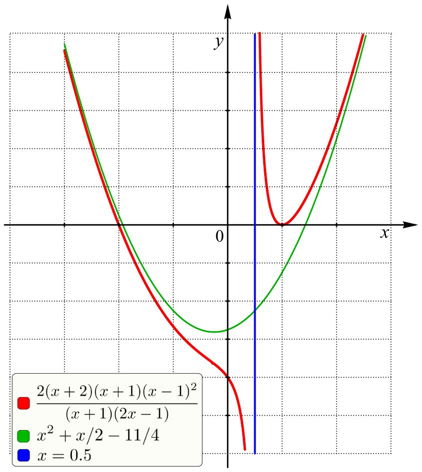
The routine
Everything in this chapter now collapses into one repeatable checklist. Work it in order. The order is not arbitrary — each step depends on the one before it, and the most common wrong graphs come from doing step 3 before step 2.
| Step | What you do | What it gives you |
|---|---|---|
| 1 | Factor the numerator and the denominator completely | Everything else depends on this |
| 2 | Set the original denominator equal to zero and solve | The domain — the excluded x-values |
| 3 | Cancel any common factors | Holes, at the cancelled x-values |
| 4 | Set the remaining denominator equal to zero | Vertical asymptotes — draw as dashed lines |
| 5 | Set the remaining numerator equal to zero | x-intercepts (discard any excluded value) |
| 6 | Evaluate f(0), if 0 is in the domain | The y-intercept |
| 7 | Compare degrees (divide if the top wins by one) | Horizontal or slant asymptote |
| 8 | Pick a test x in each region between the critical values | A sign chart: above or below the axis in each strip |
Steps 4, 5, and 6 give you the actual points and lines. Step 8 is what stops you from guessing: once you know whether the curve is above or below the axis in every strip, and which way it runs at each wall, the shape has essentially no freedom left.
Worked example — a complete graph, start to finish
Sketch f(x) = (2x2 − 2x − 12)/(x2 − 9).
Step 1 — factor. The numerator has a common factor of 2: 2x2 − 2x − 12 = 2(x2 − x − 6). Two numbers multiplying to −6 and adding to −1 are −3 and 2, so this is 2(x − 3)(x + 2). The denominator is a difference of squares: x2 − 9 = (x − 3)(x + 3). So
f(x) = [2(x − 3)(x + 2)]/[(x − 3)(x + 3)]
Step 2 — domain. The original denominator is zero at x = 3 and x = −3. Domain: all real x with x ≠ 3 and x ≠ −3.
Step 3 — cancel, and record the hole. The (x − 3) cancels, leaving f(x) = [2(x + 2)]/(x + 3) for x ≠ 3. Height of the hole: substitute x = 3 into the simplified form: [2(3 + 2)]/(3 + 3) = [2(5)]/6 = 10/6 = 5/3 ≈ 1.67. Hole at (3, 5/3) — an open circle.
Step 4 — vertical asymptote. The remaining denominator (x + 3) is zero at x = −3, and it did not cancel. Vertical asymptote: x = −3.
Step 5 — x-intercept. Set the remaining numerator to zero: 2(x + 2) = 0 gives x + 2 = 0, so x = −2. That value is in the domain, so (−2, 0) is a real intercept.
Step 6 — y-intercept. Zero is in the domain, so evaluate: f(0) = [2(0 + 2)]/(0 + 3) = [2(2)]/3 = 4/3 ≈ 1.33. (0, 4/3).
Step 7 — horizontal asymptote. Use the original: the numerator has degree 2 with leading coefficient 2, the denominator has degree 2 with leading coefficient 1. Equal degrees, so y = 2/1 = 2. Horizontal asymptote: y = 2. (The simplified form agrees: degree 1 over degree 1, leading coefficients 2 and 1, giving 2/1 = 2.)
Step 8 — sign chart. The critical values are x = −3 (asymptote) and x = −2 (intercept). They cut the line into three strips. Test one number in each:
- x = −4: [2(−4 + 2)]/(−4 + 3) = [2(−2)]/(−1) = (−4)/(−1) = 4. Positive — the curve is above the axis to the left of −3.
- x = −2.5: [2(−2.5 + 2)]/(−2.5 + 3) = [2(−0.5)]/(0.5) = (−1)/(0.5) = −2. Negative — below the axis between −3 and −2.
- x = 0: we already found 4/3. Positive — above the axis to the right of −2.
Step 9 — behavior at the wall. Approach x = −3 from the left, at x = −3.1: [2(−1.1)]/(−0.1) = (−2.2)/(−0.1) = 22, and at x = −3.01 it is (−2.02)/(−0.01) = 202. Shooting to +∞. From the right, at x = −2.9: [2(−0.9)]/(0.1) = (−1.8)/(0.1) = −18, and at x = −2.99 it is (−1.98)/(0.01) = −198. Plunging to −∞.
Step 10 — how it meets y = 2. At x = 100: [2(102)]/(103) = 204/103 ≈ 1.98 — just below 2. At x = −100: [2(−98)]/(−97) = (−196)/(−97) ≈ 2.02 — just above 2. So the right branch rises toward 2 from underneath and the left branch settles toward 2 from above.
The finished picture. Draw the dashed lines x = −3 and y = 2. On the far left the curve is slightly above y = 2, and as it moves right it climbs steeply to +∞ against the wall at x = −3. On the other side of the wall it comes up from −∞, crosses the axis at (−2, 0), passes through (0, 4/3), and flattens out toward y = 2 from below — with one open circle punched out at (3, 5/3). Every feature came from arithmetic, not guesswork.
Three habits that keep you honest
First, label the hole separately from the asymptote. Both come from the denominator, and both are excluded from the domain, but they look nothing alike: a hole is one missing dot on an otherwise ordinary curve, while an asymptote splits the graph into separate branches. Writing "x ≠ 3, x ≠ −3" tells you two values are excluded; only the factoring tells you which is which.
Second, sanity-check with one far-out number. Plug in x = 100 or x = −100 and compare against the asymptote you predicted, exactly as Step 10 did. If you predicted y = 2 and the arithmetic hands back 1.98, you are right. If it hands back 47, you made an error upstream — almost always in the degree comparison or in a dropped negative sign.
Third, when you solve rather than graph, check every candidate against the domain. Clearing fractions is legal, but it can manufacture answers the original equation never had. Solve (x + 3)/(x − 3) = 6/(x − 3) by multiplying both sides by (x − 3) and you get x + 3 = 6, so x = 3. But x = 3 was excluded from the domain from the very first line — both sides are undefined there. That candidate is extraneous, and the equation has no solution. The rule is absolute: substitute every answer back into the original equation, and throw out any value that makes a denominator zero.
The same caution applies to inequalities, but the fix is different. Do not multiply a rational inequality by a factor such as (x + 3), because you do not know its sign — and multiplying or dividing both sides of an inequality by a negative quantity reverses the inequality sign. With plain numbers that rule is easy to apply: −2x < 6 becomes x > −3, not x < −3. (Check x = 0: −2(0) = 0, and 0 < 6 is true, and 0 > −3 is true.) With a variable factor you cannot apply it, because the sign changes from strip to strip. That is precisely why Step 8 uses a sign chart instead: testing one number in each region settles the sign question without ever multiplying through.
- Follow the checklist in order: factor → domain → cancel (holes) → vertical asymptotes → intercepts → end behavior → sign chart.
- The sign chart removes the guesswork — test one x in each strip between critical values.
- Near a vertical asymptote, test a value just left and just right; the two sides often run in opposite directions.
- Confirm the horizontal or slant asymptote with a far-out value such as x = 100 before you commit to the sketch.
- When you solve a rational equation, substitute back: any candidate that makes a denominator zero is extraneous and must be discarded. For an inequality, never multiply by a variable factor — multiplying or dividing by a negative flips the inequality sign, so use a sign chart instead.
The chapter in one breath
- A polynomial allows only whole-number exponents, and its graph is continuous and smooth — no gaps, no corners.
- Degree and leading coefficient alone fix the end behavior: even degree makes the two ends agree, odd degree makes them disagree, and a negative leading coefficient flips the whole picture.
- Zeros are x-intercepts; find them by factoring completely and applying the zero-product property, then check each one by substituting.
- Odd multiplicity means the graph crosses the axis; even multiplicity means it touches and turns around. The multiplicities add up to the degree.
- Long division works for any divisor; synthetic division is the fast version reserved for divisors of the form x − c — mind the sign of c and the 0 placeholders.
- The Remainder Theorem says the remainder is P(c), and the Factor Theorem says a remainder of 0 means (x − c) is a factor — the standard way to break a cubic down to a quadratic.
- For a rational function, factor first and state the domain before cancelling: cancelled factors become holes, surviving denominator factors become vertical asymptotes.
- Degrees settle the far ends: smaller top → y = 0; equal degrees → the ratio of leading coefficients; top bigger by exactly one → a slant asymptote found by division.
- Solving is not graphing: clearing fractions can create extraneous solutions, so substitute every answer back into the original equation and discard anything that makes a denominator zero — and remember that multiplying or dividing an inequality by a negative reverses the inequality sign.
ReferenceWords worth knowing
A quick reference for the vocabulary in this chapter — skim it now, or come back whenever a term stops you mid-problem.
- Asymptote
- A line that a graph approaches more and more closely as it heads toward infinity (or toward an excluded x-value). It is drawn dashed because it is a guide, not part of the curve.
- Degree
- The highest exponent on the variable once a polynomial is written in standard form. It caps the number of zeros at n and the number of turning points at n − 1.
- Dividend
- In a division problem, the polynomial being divided — the one under the bar.
- Divisor
- The polynomial you are dividing by.
- End behavior
- What the two arms of a graph do as x → +∞ and x → −∞; for a polynomial it is decided entirely by degree and leading coefficient.
- Extraneous solution
- A value that appears when you clear fractions (or otherwise transform an equation) but does not satisfy the original equation — typically because it makes a denominator zero. Always substitute back and discard any such value.
- Factor Theorem
- (x − c) is a factor of P(x) if and only if P(c) = 0 — that is, if and only if the remainder on dividing by x − c is zero.
- Hole (removable discontinuity)
- A single missing point on an otherwise ordinary curve, caused by a factor that cancels from both numerator and denominator. Marked with an open circle.
- Horizontal asymptote
- A horizontal line y = k that the graph approaches as x → ±∞. A graph is allowed to cross it in the middle.
- Leading coefficient
- The number multiplying the highest-degree term, sign included. Its sign flips the entire end-behavior picture.
- Long division (polynomial)
- The general division algorithm — divide, multiply, subtract, bring down — that works with a divisor of any degree.
- Multiplicity
- The exponent on a repeated factor, telling you how many times a zero occurs. Odd multiplicity → the graph crosses; even multiplicity → it touches and turns.
- Polynomial function
- A sum of terms of the form a xn with n a whole number; no variables in denominators, none under radicals.
- Quotient
- The result of a division, not counting the remainder.
- Rational function
- A function written as one polynomial divided by another, P(x)/Q(x), with Q(x) not the zero polynomial.
- Remainder
- What is left over after dividing; its degree is always less than the degree of the divisor.
- Remainder Theorem
- Dividing P(x) by x − c leaves a remainder of exactly P(c) — a fast way to evaluate or to test a candidate zero.
- Slant (oblique) asymptote
- A slanted line the graph approaches at its far ends; it occurs when the numerator's degree is exactly one more than the denominator's, and you find it by dividing.
- Synthetic division
- A coefficients-only shortcut for dividing by x − c, using bring-down, multiply, add. Requires 0 placeholders for any missing power.
- Turning point
- A point where the graph changes from rising to falling or from falling to rising; a degree-n polynomial has at most n − 1 of them.
- Vertical asymptote
- A vertical line x = a that the graph races along but never touches, occurring where a denominator factor survives after cancelling.
- x-intercept
- A point (c, 0) where the graph meets the horizontal axis; the x-values are exactly the real zeros.
- Zero (root)
- A number c for which P(c) = 0. Also called a root of the equation P(x) = 0 or a solution of it.